Imbalanced data classification part1

Imbalanced_image Cute imbalanced image¹

지도학습에서 분류 문제를 다룰 때 Imbalanced classification인 경우가 많았습니다. 예를 들어 이커머스 데이터를 활용하여 개별적인 고객의 이탈을 예측하는 모델을 만들 때 위의 문제를 발견할 수 있었습니다. 실무에서 이탈 예측 태스크를 진행하면서 ‘불균형 데이터를 어떻게 다룰 것인가’에 대하여 생각한 것들을 두 개의 블로그 컨텐츠로 정리하는 시간을 가졌습니다. 해당 글은 그 중 첫번째 글입니다.

Imbalanced data

Definition of Imbalanced data

처음에는 데이터의 반응변수의 분포가 고르게 퍼진 Unbalanced data와 다르게 Imbalanced data는 도메인 특성상 내재적인 이유로 처음부터 반응변수의 분포가 왜곡된 데이터로 정의할 수 있습니다. 이러한 문제는 앞에서 언급한 ‘고객 이탈 예측’, ‘이상치 탐지’, ‘스팸 탐지’까지 다양한 상황에서 직면할 수 있습니다.

Case	심각한 불균형 O	심각한 불균형 X	충분한 데이터 샘플 O	충분한 데이터 샘플 X
case 1	O	X	O	X
case 2	O	X	X	O
case 3	X	O	O	X
case 4	X	O	X	X

각각의 케이스마다 접근 방법을 다르게 할 필요성이 있지만 특히 case 2번[심각한 불균형이면서 충분한 데이터 샘플을 확보하지 못한 경우]같은 경우는 분류 모델을 구성하기 상당히 힘듭니다. 위의 테이블에서 우리는 데이터 자체의 크기, 노이즈(Noise)를 유발하는 데이터, 그리고 왜도가 높은 데이터 분포가 특정한 분류 문제를 어렵게 만듬을 알 수 있습니다.

Evaluation Metrics of Imbalanced data classification

Three families of evaluation metrics of classification

다음의 논문²에서 분류 문제에 대한 평가 지표를 다음과 같이 세 가지로 구분하였습니다.

Threshold Metrics
Ranking Metrics
Probability Metrics

세 가지 분류 지표군들에서 Train data와 Test data간의 분포가 비슷하다고 가정할 때 사용되는 ‘Threshold Metrics’를 알아보겠습니다.

Threshold Metrics

‘Threshold Metrics’는 분류 예측 모델의 오분류를 정량화한 지표입니다. 다음과 같은 표를 많이 보셨을 겁니다.

	Positive Prediction	Negative Prediction
Positive Class	TP(True Positive)	FN(False Negative)
Negative Class	FP(False Positive)	TN(True Negative)

이커머스에서 이탈 예측 문제를 해당 표와 연결하면 다음과 같습니다.

	이탈로 예측	이탈이 아니라고 예측
실제 이탈 O	TP(True Positive)	FN(False Negative)
실제 이탈 X	FP(False Positive)	TN(True Negative)

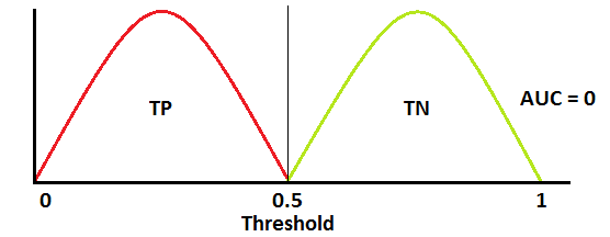
사기 탐지(Fraud detection) 영역에서는 다음과 같은 그림으로 위의 표의 케이스를 응용하여 해석할 수 있습니다.

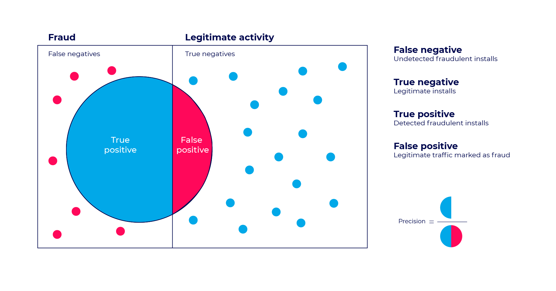false-positive-test-diagram false-positive test diagram in fraud detection³

\[Accuracy = \frac {TP + TN}{TP+FN+FP+TN}\]

\[Error = 1 - Accuracy = \frac {FP + FN}{TP+FN+FP+TN}\]

Sensitivity-Specificity Metrics

일반적인 분류 문제에서는 정확도를 많이 참고합니다. 하지만 사기 탐지 데이터와 같이 극단적으로 불균형된 데이터인 경우 정확도는 크게 의미가 없습니다. FN(False Negative)와 FP(False Postivie) 모두 예측 모델이 틀린 경우들이지만 사기 탐지인 경우 FN일 때가 FP인 경우보다 훨씬 치명적입니다.
이것을 한번 위의 표와 엮으면 다음과 같은 지표를 고안하여 해석할 수 있습니다.

\[Sensitivity = \frac {TP}{TP+FN}\]

\[Specificity = \frac {TN}{FP+TN}\]

사기 탐지 같은 경우 민감도를 특이도보다 더 중요한 지표로 삼을 것입니다. 이 해석을 제가 마주한 문제에 그대로 비유하면 이탈을 하지 않는데 이탈을 하는 것으로 예측하는 것이 미래 시점에 이탈이 발생했는데 잘못 예측하는 것보다 덜 치명적일 것입니다. 하지만 일반적으로 이탈하는 고객이 이탈하지 않는 고객보다 훨씬 많습니다. 그러므로 기계적인 해석이 아니라 해당 이커머스 업체의 특성에 따라서 특이도와 민감도의 차이를 비교해야 합니다.

만약 특이도와 민감도 두 가지 모두를 고려하고 싶을 때는 두 지표의 기하평균인 G-mean을 사용합니다.

\[G-mean = \sqrt{Sensitiviy \times Specificity}\]

ROC curve

ROC curve는 양성 클래스의 이진 분류 모델의 성능을 요약해주는 그래프입니다. X축은 FPR(False Positive Rate)이고 Y축은 TPR(True Positive Rate)입니다. 먼저 TPR과 FPR을 살펴 보겠습니다.

\[TPR = \frac {TP}{TP+FN}\]

\[FPR = \frac {FP}{FP+TN}\]

TPR은 양성 클래스를 얼마나 잘 예측한지를 알려줍니다.FPR은 전체 음성 클래스에서 양성으로 잘못 예측할 비율을 의미합니다. TPR을 FPR로 나눴을 경우 다음과 같습니다.

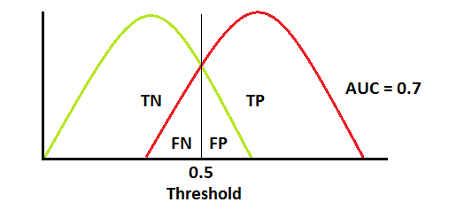
\[\frac{(\frac {TP}{TP+FN})}{(\frac {FP}{FP+TN})} = \frac{TP \times (FP+TN)}{ FP \times (TP+FN)}\]

양성 클래스(TP+FN)와 음성 클래스(FP+TN)는 이미 상수이므로 ROC값을 변화시키는 것은 TP와 FP입니다. 하지만 TP와 FP는 Threshold에 따라 달라집니다. 그러므로 실제 클래스 및 모델 예측값의 분포 관계에 따라서 ROC AUC를 다음과 같이 그릴 수 있을 것입니다.

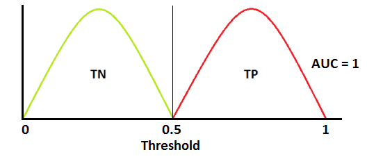ROC_curve_best1 Best ROC curve dist⁴ 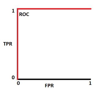ROC_curve_best2 Best ROC AUC

ROC_curve_mid1 General curve dist 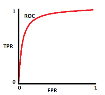ROC_curve_mid2 General ROC AUC

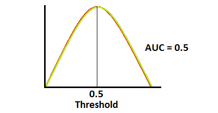ROC_curve_501 ROC half curve dist 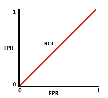ROC_curve_502 half ROC UC

ROC_curve_worst1 ROC worst curve dist 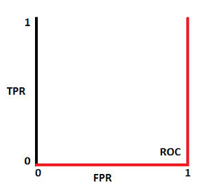ROC_curve_worst2 Worst ROCAUC

Precision-Recall Metrics

수식상으로 Precision과 Recall을 살펴보면 다음과 같습니다.

\[Precision = \frac {TP}{TP+FP}\]

\[Recall = \frac {TP}{TP+FN}\]

수식의 의미를 사기 탐지 태스크와 이탈 예측 태스크에 각각 맞추어서 살펴보겠습니다. 사기 탐지 태스크에서 정밀도의 의미는 해당 클래스가 ‘사기’로 예측하였을 때 실제로 사기일 비율을 의미합니다. 이와 유사하게 이탈 예측 태스크에서 정밀도의 의미는 해당 클래스가 ‘이탈’로 예측하였을 때 실제로 ‘이탈’을 할 비율을 뜻합니다.

재현율은 수식상으로 민감도와 같습니다. 사기 탐지 태스크에서 재현율은 해당 클래스가 실제로 ‘사기’일 때 사기로 예측할 확률을 말합니다. 이탈 예측 태스크에서는 실제로 ‘이탈’일 때 이탈로 예측할 비율을 의미합니다.

수식에서 알 수 있듯이 정밀도와 재현율의 관계는 다음과 같습니다.

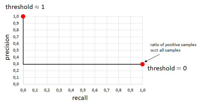
\[\frac{(\frac {TP}{TP+FP})}{(\frac {TP}{TP+FN})} = \frac{TP \times (TP+FN)}{ TP \times (TP+FP)} = \frac{TP+FN}{TP+FP}\]

ROC curve와 마찬가지로 Threshold를 설정함에 따라서 값이 달라집니다. 하지만 음성 클래스와 양성 클래스를 모두 고려하는 ROC curve와 다르게 PR curve는 소수 클래스인 양성 클래스만을 고려합니다. 이 점을 고려할 때 실무적으로 굉장히 Skewed한 클래스 분포를 가지면서 ROC AUC가 너무 높은 값을 가졌을 때 소수 클래스에 초점을 맞춘 PR AUC를 확인하여 분류 모델의 성능을 종합적으로 확인할 수 있습니다.

Recall-Precision을 그래프로 그리고 다음과 같은 경우가 있을 것입니다.

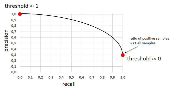Precision_Recall_Curve_image1 General Precision-Recall Curve⁵

모델의 성능이 아주 뛰어나거나 안좋으면 다음과 같이 그려질 것입니다.

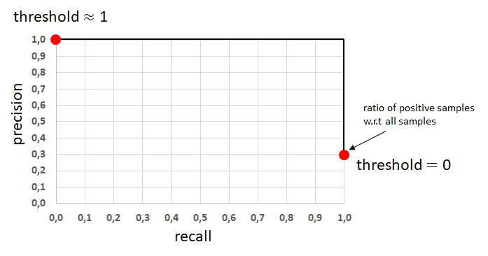Precision_Recall_Curve_image2 Best Precision-Recall Curve

Precision_Recall_Curve_image3 Worst Precision-Recall Curve

Data sampling

데이터 샘플링은 반응 변수의 분포를 유지시키기 위한 방법입니다. 예측 모델을 신중히 선택하는 만큼 다양한 데이터 샘플링 기법들 중 가장 자신의 문제 상황에 맞는 방법을 결정해야 합니다.
만약 데이터가 왜곡되어 있다면 많은 머신러닝 모델들은 다수를 차지하는 클래스에서 관측되는 예측 변수들의 가능도에 초점이 맞추어 질 것입니다.
이런 경우, 이탈 예측과 같이 소수 클래스와 예측 변수들의 관계를 포착하는 것이 중요한 태스크는 예측 모델을 구성할 때 심각한 문제에 직면할 수 있습니다.

Random sampling

Random Undersampling

학습 데이터 세트에서 다수 클래스를 랜덤하게 선택한 후 지우는 샘플링 기법입니다.
불균형한 데이터이지만 소수를 차지하는 클래스가 충분한 관측치를 가지고 있는 경우 사용합니다.
다만 Undersampling 기법의 특성상 다수의 클래스에서 지워지는 데이터가 분류 경계를 짓는데 아주 중요할 경우 예측 모델 정확도가 떨어질 수 있습니다.

RUS에 대한 이미지를 살펴보면 다음과 같습니다.

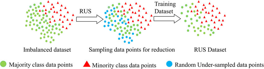random_undersampling_image RUS⁶

Random Oversampling

소수 클래스의 데이터 중에서 일정한 수를 랜덤하게 선택하여 다수 클래스의 수만큼 복제하는 기법입니다.
왜곡된 분포에 크게 영향을 받는 머신러닝 모델에 적합하지만 소수의 클래스에 과적합이 발생하여 일반화에 악영향을 끼칠 수 있습니다.
만약 다수 클래스의 데이터가 엄청 클 경우 Oversampling된 후의 데이터를 학습시킬 때 계산 속도가 오래 걸립니다.
이런 악영향을 방지하기 위해서 Raw data에 예측 모델과 Random Oversapling을 적용한 데이터에 적합시킨 예측 모델간의 성능을 비교할 필요가 있습니다.

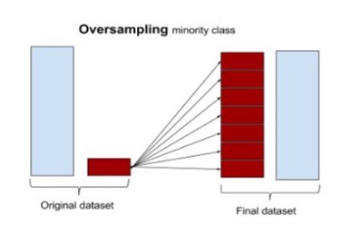random_oversampling_image ROS⁷

Undersampling

단순히 다수 클래스의 샘플 수를 랜덤하게 뽑아서 제거하는 것이 아닌 일정한 논리에 따라 데이터의 Feature Space를 최대한 유지시키는 방향으로 UnderSampling을 진행할 수 있습니다.
먼저 다음의 상황을 가정해 봅니다.
- 아래의 표는 개별적인 특성이 담긴 테이블입니다.
- 다음과 같은 기준으로 사람들을 묶을 수 있을 것입니다.
  - 비슷한 특질이 있는 사람들 끼리 묶기!
  - 비슷하지 않는 특색을 가진 사람들을 구분하기!
  - 첫번째 방법과 두번째 방법을 섞어서 묶기!

Feature	Lee	Koo	Kwon	Kim	Ko	Cho	Oh
Feature_a	O	O	O	O	O	X	X
Feature_b	O	O	X	X	X	O	O
Feature_c	X	X	O	O	O	X	X

Undersampling도 앞의 세 가지 경우와 비슷합니다. 구체적으로 다음과 같이 기법을 세분화할 수 있습니다. 세부적인 Sampling 기법의 방법들에 대해 알고 싶으시면 아래 주석의 논문들을 참고하시길 바랍니다.

유지할 데이터를 선택하는 방법
- Near Miss Undersampling⁸
  - NearMiss-1 : 소수 클래스로부터 다수 클래스의 샘플들 중 가장 평균 거리가 작은 k개의 샘플을 뽑습니다.
  - NearMiss-2 : 소수 클래스로부터 다수 클래스의 샘플들 중 가장 평균 거리가 먼 k개의 샘플을 뽑습니다.
  - NearMiss-3 : 소수의 클래스의 개별 샘플로부터 가장 거리가 가까운 샘플들을 뽑습니다.
- Condensed Nearest Neighbor Rule⁹
  - CNN기법은 모델의 성능에 해를 끼치지 않는 데이터의 부분집합을 찾는 방법입니다.
  - 자세한 내용은 아래의 코드와 함께 설명하였습니다.
제거할 데이터를 선택하는 방법
- Tomek Links¹⁰
- ENN(Edited Nearest Neighbor Rule)¹¹
첫번째와 두번째를 적절히 섞은 방법
- One-Sided Selection¹²
  - Tomek Links -> CNN
- Neighborhood Cleansing Rule¹³
  - CNN -> ENN

유지할 데이터를 선택하는 방법

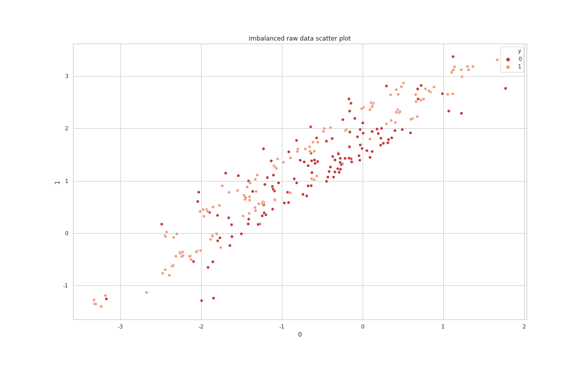
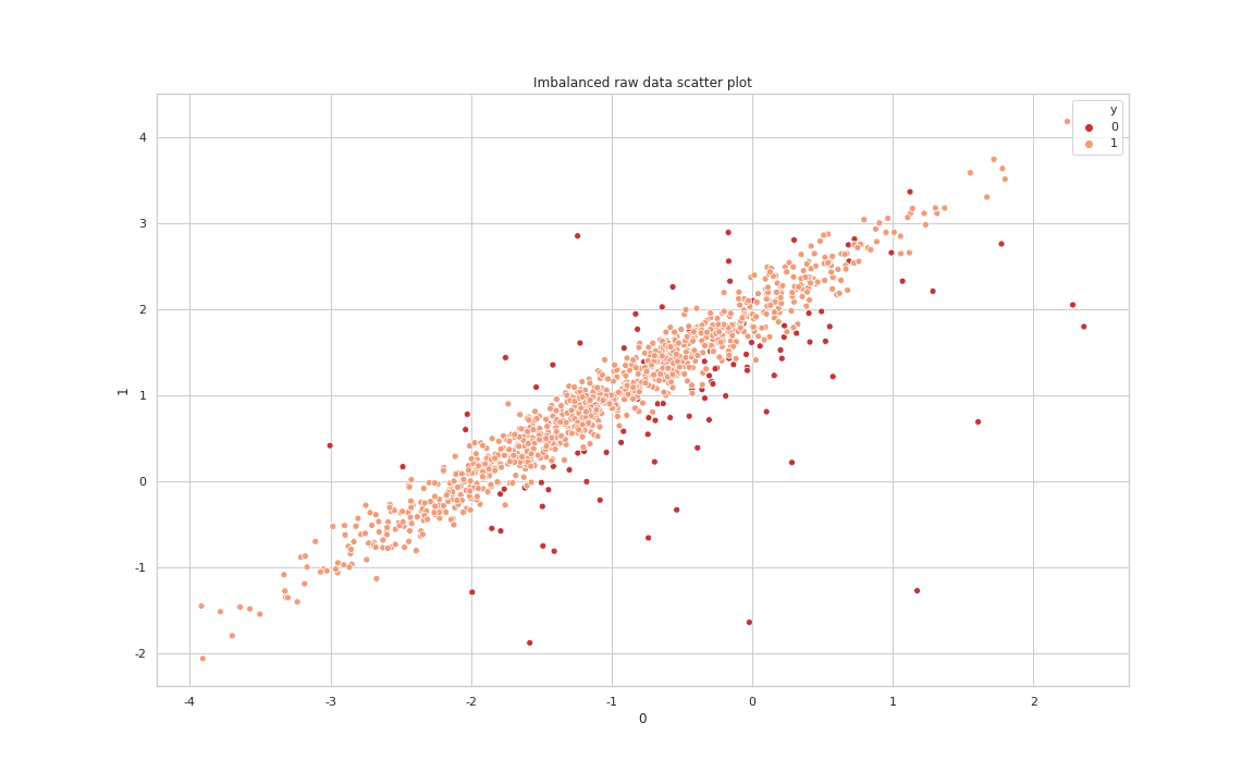
가상의 불균형 데이터를 만들어서 Under sampling의 효과를 살펴보겠습니다. 먼저 10000개 샘플에 관하여 두 가지 예측 변수들과 클래스가 0이거나 1인 클래스를 구성하겠습니다. 노이즈 데이터의 비율은 실험의 명확성을 위해 0으로 설정하였고 다수 클래스에 대한 가중치는 90%로 설정하였습니다.

X, y = mc(n_samples=10000,
		 weights=[0.90],
                n_features = 2,
                n_redundant=0,
                n_clusters_per_class=1,
                random_state = 33,
                flip_y=0)

print(Counter(y))

Counter({0: 9001, 1: 999})

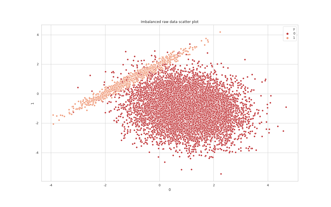raw_data_scatter_plot Raw data Scatter Plot

Nearmiss-3

다수 클래스와 소수 클래스의 Boundary를 알 수 있게 해주는 “NearMiss-3” 기법[각각의 소수 클래스로부터 거리가 가까운 다수 클래스내 샘플 수 기준은 5입니다]을 적용한 데이터의 Scatter plot을 살펴보면 다음과 같습니다.

nearmiss_plot Nearmiss3 data Scatter Plot

Condensed nearest neighbour

다음은 imbalanced-learn library에서 Condensed nearest neighbour¹⁴를 구현한 코드입니다. 코드 내용을 통해 CNN은 다음과 같이 동작함을 알 수 있습니다.

Random Seed를 설정한 후 다수 클래스에서 하나의 샘플을 임의적으로 추출합니다.
모든 소수 클래스의 샘플들과 앞에서 추출한 샘플을 사용하여 하나의 부분집합(C)을 생성합니다.
모든 다수 클래스를 이용하여 부분집합 S를 만듭니다.
Set C를 KNN에 적합시킨 후 모델이 제대로 분류한 샘플들은 고르지 않고 제대로 분류되지 않은 샘플들을 C에 Append시킵니다.
해당 알고리즘은 이중 for문을 쓰는 구조이므로 knn의 하이퍼 파라미터를 작게 해주는 것이 일반적으로 좋습니다.

def _fit_resample(self, X, y):
    self._validate_estimator()

    random_state = check_random_state(self.random_state)
    target_stats = Counter(y)
    class_minority = min(target_stats, key=target_stats.get)
    idx_under = np.empty((0,), dtype=int)

    for target_class in np.unique(y):
        if target_class in self.sampling_strategy_.keys():
            # Randomly get one sample from the majority class
            # Generate the index to select
            idx_maj = np.flatnonzero(y == target_class)
            idx_maj_sample = idx_maj[
                random_state.randint(
                    low=0,
                    high=target_stats[target_class],
                    size=self.n_seeds_S,
                )
            ]

            # Create the set C - One majority samples and all minority
            C_indices = np.append(
                np.flatnonzero(y == class_minority), idx_maj_sample
            )
            C_x = _safe_indexing(X, C_indices)
            C_y = _safe_indexing(y, C_indices)

            # Create the set S - all majority samples
            S_indices = np.flatnonzero(y == target_class)
            S_x = _safe_indexing(X, S_indices)
            S_y = _safe_indexing(y, S_indices)

            # fit knn on C
            self.estimator_.fit(C_x, C_y)

            good_classif_label = idx_maj_sample.copy()
            # Check each sample in S if we keep it or drop it
            for idx_sam, (x_sam, y_sam) in enumerate(zip(S_x, S_y)):

                # Do not select sample which are already well classified
                if idx_sam in good_classif_label:
                    continue

                # Classify on S
                if not issparse(x_sam):
                    x_sam = x_sam.reshape(1, -1)
                pred_y = self.estimator_.predict(x_sam)

                # If the prediction do not agree with the true label
                # append it in C_x
                if y_sam != pred_y:
                    # Keep the index for later
                    idx_maj_sample = np.append(
                        idx_maj_sample, idx_maj[idx_sam]
                    )

                    # Update C
                    C_indices = np.append(C_indices, idx_maj[idx_sam])
                    C_x = _safe_indexing(X, C_indices)
                    C_y = _safe_indexing(y, C_indices)

                    # fit a knn on C
                    self.estimator_.fit(C_x, C_y)

                    # This experimental to speed up the search
                    # Classify all the element in S and avoid to test the
                    # well classified elements
                    pred_S_y = self.estimator_.predict(S_x)
                    good_classif_label = np.unique(
                        np.append(
                            idx_maj_sample, np.flatnonzero(pred_S_y == S_y)
                        )
                    )

            idx_under = np.concatenate((idx_under, idx_maj_sample), axis=0)
        else:
            idx_under = np.concatenate(
                (idx_under, np.flatnonzero(y == target_class)), axis=0
            )

    self.sample_indices_ = idx_under

    return _safe_indexing(X, idx_under), _safe_indexing(y, idx_under)

앞의 불균형 데이터에 CNN[k value in KNN = 5]을 적용하면 다음과 같습니다.

Raw data --> Counter({0: 9001, 1: 999})
After CNN processing --> Counter({0: 153, 1: 999})

CNN After CNN processing data Scatter Plot

CNN은 Under sampling 기법 중 ‘유지할 데이터를 선택하는 방법’에 충실하지만 다음과 같은 코드에서 임의성을 발견할 수 있습니다.

for target_class in np.unique(y):
        if target_class in self.sampling_strategy_.keys():
            # Randomly get one sample from the majority class
            # Generate the index to select
            idx_maj = np.flatnonzero(y == target_class)
            idx_maj_sample = idx_maj[
                random_state.randint(
                    low=0,
                    high=target_stats[target_class],
                    size=self.n_seeds_S,
                )
            ]

제거할 데이터를 선택하는 방법

Tomek Links

이런 초반의 임의성은 유지하지 않아도 되는 데이터를 부분집합에 속하게 만듭니다. 이것을 제어하기 위해서 엄밀한 쌍을 하나 만듭니다. 그 쌍은 다음과 같이 정의됩니다

Tomek Link : 인스턴스 a와 인스턴스 b는 다음과 같을 때 ‘Tomek Link’라 한다. 인스턴스의 가장 가까운 이웃은 인스턴스 b이다. 마찬가지로 인스턴스 b와 가장 가까운 이웃은 인스턴스 a이다. 이 때 인스턴스 a와 인스턴스 b는 서로 다른 클래스에 속해야 한다.

이렇게 되면 앞의 CNN의 임의성을 제거되면서 각 클래스간의 경계를 명확히 알 수 있습니다. TomekLink(k = 2)의 결과를 확인해 보겠습니다.

Counter({0: 9001, 1: 999})
Counter({0: 8953, 1: 999})

After TomekLink processing data Scatter Plot

위의 그래프를 통해 알 수 있듯이 각 클래스의 경계를 아는 것만으로는 Undersampling의 큰 효과를 발휘할 수 없습니다. 그래서 실무상에서는 Tomek Link를 통해 Noise와 경계값을 제거한 후 다른 Under Sampling(Ex : CNN) 기법을 같이 사용합니다. 두 가지 기법(Tomek Link + CNN)을 같이 사용한 결과는 다음과 같습니다.

Tomek_and_CNN After TomekLink & CNN processing data Scatter Plot

Oversampling

Oversampling 기법은 불균형 데이터의 분포를 처리할 때 소수 클래스를 다수 클래스의 샘플 수에 맞추어 늘리는 방법입니다.
제일 간단한 방법은 소수 클래스의 샘플을 단순하게 복제하는 것입니다. 다만 이럴 경우 학습하려는 모델에 어떤 새로운 정보를 제공할 수 없습니다.
대신에 소수 클래스에 대하여 새로운 정보를 주면서 augmentation하는 기법 중 SMOTE(Synthetic Minority Oversampling Technique)¹⁵가 있습니다.

SMOTE

다음은 imbalanced-learn library에서 SMOTE를 구현한 코드입니다. 위의 논문 및 Borderline 관련 추가 논문¹⁶과 코드를 통해 SMOTE는 다음과 같이 동작함을 알 수 있습니다.

먼저 소수 클래스의 샘플들을 랜덤으로 선택합니다.
선택된 임의의 개별적인 샘플[S1]에서 Featrue Space에서 거리가 가장 가까우면서 소수 클래스에 속한 k개의 샘플들[S2]을 선택합니다.
S1과 S2를 직선으로 연결한 후 그 직선상에서 새로운 데이터를 생성합니다.
- 일반적으로 직선상에 생성된 샘플은 직선과 거리가 먼 샘플보다 오분류가 될 가능성이 더 높습니다.
- 다시 말해서 거리가 먼 샘플들은 KNN 알고리즘에 따라소수 클래스보다 다수 클래스에 속할 가능성이 높을 때 오분류의 가능성이 높은 Danger 샘플로 간주됩니다.
  - borderline-SMOTE1 : Danger 샘플과 소수 클래스 간의 거리차이의 가중치를 0~1로 줍니다.
  - borderline-SMOTE2 : Danger 샘플과 소수 클래스 간의 거리차이의 가중치를 0~0.5로 줍니다. 그래서 ‘borderline-SMOTE1’보다 더 가까운 샘플들을 생성합니다.
- 신기하게도 SMOTE 알고리즘의 객체를 소수 클래스가 아닌 다수 클래스에 적용을 해도 같은 현상이 발견될 수 있습니다.

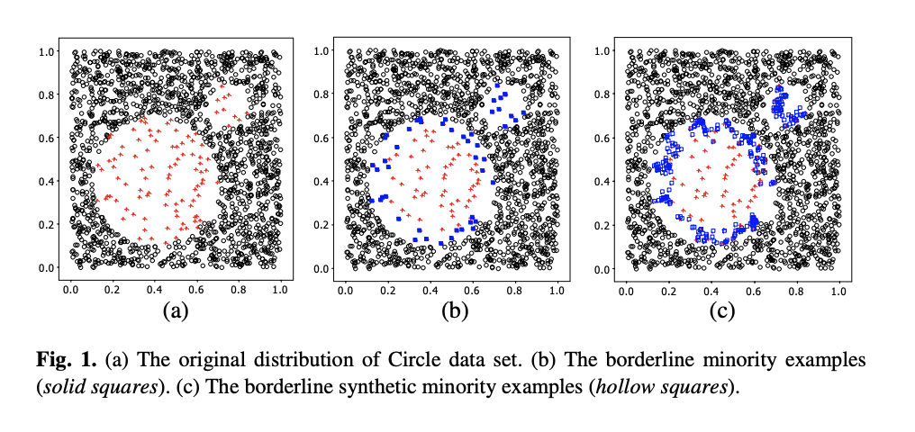SmoteImage SMOTE Image

def _validate_estimator(self):
    super()._validate_estimator()
    self.nn_m_ = check_neighbors_object(
        "m_neighbors", self.m_neighbors, additional_neighbor=1
    )
    self.nn_m_.set_params(**{"n_jobs": self.n_jobs})
    if self.kind not in ("borderline-1", "borderline-2"):
        raise ValueError(
            'The possible "kind" of algorithm are '
            '"borderline-1" and "borderline-2".'
            "Got {} instead.".format(self.kind)
        )

def _fit_resample(self, X, y):
    self._validate_estimator()

    X_resampled = X.copy()
    y_resampled = y.copy()

    for class_sample, n_samples in self.sampling_strategy_.items():
        if n_samples == 0:
            continue
        target_class_indices = np.flatnonzero(y == class_sample)
        X_class = _safe_indexing(X, target_class_indices)

        self.nn_m_.fit(X)
        danger_index = self._in_danger_noise(
            self.nn_m_, X_class, class_sample, y, kind="danger"
        )
        if not any(danger_index):
            continue

        self.nn_k_.fit(X_class)
        nns = self.nn_k_.kneighbors(
            _safe_indexing(X_class, danger_index), return_distance=False
        )[:, 1:]

        # divergence between borderline-1 and borderline-2
        if self.kind == "borderline-1":
            # Create synthetic samples for borderline points.
            X_new, y_new = self._make_samples(
                _safe_indexing(X_class, danger_index),
                y.dtype,
                class_sample,
                X_class,
                nns,
                n_samples,
            )
            if sparse.issparse(X_new):
                X_resampled = sparse.vstack([X_resampled, X_new])
            else:
                X_resampled = np.vstack((X_resampled, X_new))
            y_resampled = np.hstack((y_resampled, y_new))

        elif self.kind == "borderline-2":
            random_state = check_random_state(self.random_state)
            fractions = random_state.beta(10, 10)

            # only minority
            X_new_1, y_new_1 = self._make_samples(
                _safe_indexing(X_class, danger_index),
                y.dtype,
                class_sample,
                X_class,
                nns,
                int(fractions * (n_samples + 1)),
                step_size=1.0,
            )

            # we use a one-vs-rest policy to handle the multiclass in which
            # new samples will be created considering not only the majority
            # class but all over classes.
            X_new_2, y_new_2 = self._make_samples(
                _safe_indexing(X_class, danger_index),
                y.dtype,
                class_sample,
                _safe_indexing(X, np.flatnonzero(y != class_sample)),
                nns,
                int((1 - fractions) * n_samples),
                step_size=0.5,
            )

            if sparse.issparse(X_resampled):
                X_resampled = sparse.vstack(
                    [X_resampled, X_new_1, X_new_2]
                )
            else:
                X_resampled = np.vstack((X_resampled, X_new_1, X_new_2))
            y_resampled = np.hstack((y_resampled, y_new_1, y_new_2))

    return X_resampled, y_resampled

위와 같은 순서로 말미암아 다음과 같이 SMOTE의 장단점을 찾을 수 있습니다.
- 새로운 정보를 제공해서 학습시키려는 모델이 결정 경계를 효율적으로 배울 수 있도록 합니다.
- 단순히 Undersampling 기법만 적용한는 것보다 SMOTE와 Under Sampling을 같이 활용할 때 모델 성능이 올라갑니다.
- 음성 클래스와 양성 클래스의 예측값과 실제값의 분포가 많이 겹칠 경우 SMOTE를 통한 오버샘플링된 샘플들이 오히려 결정 경계를 모호하게 만들 수 있습니다.

ADASYN

Mixed Sampling

SMOTE + Tomek Links
SMOTE + Edited Nearest Neighbor Rule

Reference

https://medium.com/@kr.vishwesh54/a-creative-way-to-deal-with-class-imbalance-without-generating-synthetic-samples-4cfad099d405 ↩
https://www.math.ucdavis.edu/~saito/data/roc/ferri-class-perf-metrics.pdf ↩
https://towardsdatascience.com/understanding-auc-roc-curve-68b2303cc9c5 ↩
https://www.appsflyer.com/blog/click-flooding-detection-false-positive-challenge/ ↩
https://towardsdatascience.com/gaining-an-intuitive-understanding-of-precision-and-recall-3b9df37804a7 ↩
https://www.researchgate.net/figure/llustration-of-random-undersampling-technique_fig3_343326638 ↩
https://medium.com/@patiladitya81295/dealing-with-imbalance-data-1bacc7d68dff10302/24590&hl=ko&sa=X&ei=xSoBYJS3GpCbywTT47Uw&scisig=AAGBfm0zNdcfXdPynWxoQ3FsFum2KdF9ow&nossl=1&oi=scholarr ↩
https://www.site.uottawa.ca/~nat/Workshop2003/jzhang.pdf ↩
https://ieeexplore.ieee.org/document/1054155 ↩
https://ieeexplore.ieee.org/document/4309452 ↩
https://ieeexplore.ieee.org/document/4309137 ↩
https://sci2s.ugr.es/keel/pdf/algorithm/congreso/kubat97addressing.pdf ↩
https://link.springer.com/chapter/10.1007/3-540-48229-6_9 ↩
https://github.com/scikit-learn-contrib/imbalanced-learn/blob/master/imblearn/under_sampling/_prototype_selection/_condensed_nearest_neighbour.py ↩
http://scholar.google.co.kr/scholar_url?url=https://www.jair.org/index.php/jair/article/download/ ↩
http://citeseerx.ist.psu.edu/viewdoc/download?doi=10.1.1.308.9315&rep=rep1&type=pdf ↩

Imbalanced data classification part1

Imbalanced data

Definition of Imbalanced data

Evaluation Metrics of Imbalanced data classification

Three families of evaluation metrics of classification

Threshold Metrics

Sensitivity-Specificity Metrics

ROC curve

Precision-Recall Metrics

Data sampling

Random sampling

Random Undersampling

Random Oversampling

Undersampling

유지할 데이터를 선택하는 방법

Nearmiss-3

Condensed nearest neighbour

제거할 데이터를 선택하는 방법

Tomek Links

Oversampling

SMOTE

ADASYN

Mixed Sampling

Reference

Contents

Trending Tags

Imbalanced data classification part1

Imbalanced data

Definition of Imbalanced data

Evaluation Metrics of Imbalanced data classification

Three families of evaluation metrics of classification

Threshold Metrics

Sensitivity-Specificity Metrics

ROC curve

Precision-Recall Metrics

Data sampling

Random sampling

Random Undersampling

Random Oversampling

Undersampling

유지할 데이터를 선택하는 방법

Nearmiss-3

Condensed nearest neighbour

제거할 데이터를 선택하는 방법

Tomek Links

Oversampling

SMOTE

ADASYN

Mixed Sampling

Reference

Contents

Further Reading

Imbalanced data classification part2

Spark Tuning과 관련된 몇 가지 발견들

CRM 최적화 프로젝트 - 쿠폰 발급 최적화

Trending Tags